All experience and empirical data point the same way: go big on transmission pipes and stay lean on distribution pipes.
By Alexander Schou, Project Manager, Energy Plants and Infrastructure, COWI and Rune Tonell, Leading Project Manager, Energy Transition Advisory, COWI
Published in Hot Cool, edition no. 5/2026 | ISSN 0904 9681 |
District heating pipes are built to last 50 years or more. Over that time, almost everything behind the original sizing decision can change. Neighbourhoods grow, buildings become better insulated, the service might expand, supply temperatures might decrease, and new heat sources appear in places nobody had mapped when the first pipes went into the ground.
Separate local networks may even end up being connected to share production & storage capacity and spread risk. A transmission pipe sized “correctly” for today’s conditions is, almost by definition, sized for a system that will look very different in the future.
Thinking long term means accepting that some pipes get paid for before their own numbers add up – because their real value isn’t in today’s business case, but in the option they create: to densify, expand, connect, and reach better heat sources when the moment comes.
Holistic Thinking
Denmark’s success with district heating is usually credited to its technology, but part of the story is this: at its best, heat planning has treated whole cities as a single continuous project, with the backbone – the transmission pipes – sized for where the system is heading, not only for where it stands today.
When building a new network, there are two basic options for the backbone:
› Scenario A – size it “tightly” to today’s needs and upgrade it later if needed
› Scenario B – size it for the long-term plan from the outset
The central question is simple: which option is cheaper over the life of the asset?
Scenario A – Sizing the backbone tightly and upgrading later if needed
In general, the cost of a pipe can be split into two parts: C_pipe, which covers the pipe itself, including supply, fittings, valves and joints; and C_other, which covers everything else (civil works and installation, including excavation, soil disposal, backfilling, reinstatement, traffic management, welding, jointing and testing).
If the utility sizes tightly now and later has to upgrade – with probability p, after t years, at discount rate r – the expected cost of sizing the backbone tightly and upgrading later if needed C_tight, can be expressed as:

Where D0 is today’s (“tight”) dimension and D1 is the larger and upgraded dimension.

with L being the service life of the pipe.
Put simply, the entire formula tells you that you pay for the tight-dimensioned pipe now, plus a bit extra to cover the risk that you’ll have to upgrade it to a larger pipe later.
The last term in the equation expresses today’s value of the cost of upgrading at a later point in time. It takes the cost of upgrading to the larger dimension (civil works plus pipe), less the scrap value of the new pipe under straight-line depreciation, weights this by the probability that the upgrade is actually needed, and discounts the result back to present value over the number of years until the upgrade would occur. The nominal pipe costs are assumed to remain unchanged throughout the entire service life.
Scenario B – Sizing the backbone for the future
The cost of sizing the backbone for the future C_future, today, can be expressed as:
Future-proof sizing is the better bet whenever C_future is smaller than C_tight – that is, whenever:

A real-world example
Consider a 2 km transmission line, built two ways.
Scenario A uses a DN150 twin pipe – a single insulated casing carrying both the supply and return pipes – sized tightly to today’s load.
Scenario B sizes the same transmission line one step larger, DN200, to match the long-term plan.
From a specific COWI reference project in a sub-urban area, the pipe supply cost C_pipe for a DN150 is €395/m, while the remaining civil works and installation costs C_other amount to €1,630/m. This shows that the cost driver is not the pipe itself; it is the excavation, soil disposal, backfilling, reinstatement, traffic management, welding, and testing. In this example, these costs constitute approximately 80% of the total transmission line costs.
It should be noted that civil works and installation costs C_other for a district heating pipe are highly dependent on whether the area is rural or urban. In a rural area, civil works and installation costs typically make up a much smaller share than 80%, since rural areas tend to be less congested with existing underground infrastructure, can have unpaved surfaces, and benefit from cheaper traffic management, among other factors.
For the same reference project, the pipe supply cost C_pipe for a DN200 is €587/m, i.e. a unit cost premium of about 49% more for a DN200, compared to the DN150.
The interesting point, and the key point here, is that the remaining civil works and installation cost C_other for a DN200 amounts to only €1,697/m, equivalent to an increase of just 4%.
This means the weighted-average extra cost of stepping up from DN150 to DN200 is only app. 13% in this case. In return, that same step-up delivers an increased capacity of app. 69% – calculated as a simple ratio between the cross-sectional areas – assuming no changes in the allowed pressure gradient or velocity of the water.
Whether scenario A or B is the preferred solution financially, of course depends on the probability p that an upgrade is needed and the number of years t before it happens. For this example, the table below shows the calculations. The tendency is clear: tight sizing only comes out ahead when the probability of needing more capacity is low, or when the upgrade is decades away.
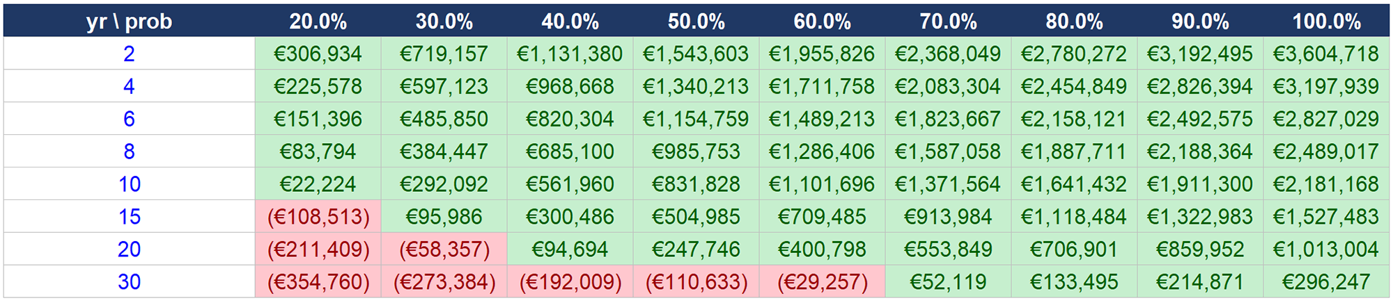
Table 1 – Expected lifetime CAPEX advantage of oversizing a 2 km backbone with 1 dimension (from DN150 to DN200), as a function of years until upgrade and probability that the upgrade is needed. Green = oversizing wins. Red = tight-sizing wins. The assumed discount rate is 3.5%, and the service life is 60 years.
The table clearly shows that sizing tightly and revisiting the pipe later can easily end up being the most expensive choice – making the case for holistic planning and modest future-ready sizing clear.
In addition, upgrading later means reopening a street to replace a functioning transmission line. It can disrupt supply to existing customers and delay the development, additional heat demand, or new heat source that the upgrade was meant to enable. To keep the calculation simple, these impacts are deliberately omitted.
However, this does not mean every pipe should be sized for future capacity. Local distribution pipes and the connections to individual buildings are the opposite case. They are cheap and fast to install, so there is little (if any) reason to build in spare capacity up front; they can simply be extended, street by street, as new customers connect.
A practical and technical window
The main message of this article is: “Build transmission pipes as large as reasonably possible and distribution pipes as small as practically possible”. That framing is deliberately exaggerated.
The upper limit of the window
Of course, there is an upper limit. The example in this article illustrates the expected benefit of stepping up one pipe dimension but jumping four or five dimensions introduces a different set of problems entirely. Beyond being clearly unnecessary, available underground space also imposes a physical constraint. Finally, if the diameter is too large, low-demand periods can reduce flow velocities and cause water stagnation, increasing heat losses.
On the other hand, heat loss scales with the pipe’s diameter, while the energy it carries scales with the diameter squared. So, the relative heat loss per MWh delivered actually falls as diameter grows, provided the pipe is well loaded. Oversizing only creates a heat-loss penalty while the pipe is still lightly loaded – in the early years before anticipated demand arrives. That is a transitional cost, not a permanent one.
The lower limit of the window
Choosing too small a diameter, on the other hand, creates trouble much faster on the hydraulic side. Halving the diameter roughly quadruples the velocity. Pressure loss is hit even harder. By the Darcy–Weisbach formula, it scales roughly with the fifth power of the diameter. Go just one size too small, and pumping costs explode. This is the main reason behind the usual design limits of around 100 Pa/m and velocities under roughly 2 m/s – and why undersizing bites so quickly.
Given the above, it is reasonable to assume that going up one or two dimensions does not raise OPEX – on the contrary, provided the pipe is well loaded, pumping costs fall. For this reason, looking at costs from a CAPEX standpoint alone, as this article does, should be sufficient for a FID.
Making the backbone affordable today
Long-term thinking requires an investment logic that openly accepts that some pipes are paid for ahead of their local business case, because their value lies in the optionality they create for the system as a whole: the ability to densify, expand, connect, and reach better heat sources when the opportunity arises.
None of this works if each neighbourhood connection must justify its own future-ready transmission line in isolation. It works when a city-wide heat plan treats the urban area as a single project delivered in phases, with a backbone sized to the long-term plan. As new neighbourhoods connect, they can then pay their share of the cost instead of placing the full burden on whoever happens to build first.
COWI’s experience is that tight dimensioning of backbones for new district heating networks often becomes more expensive over time – not only in Denmark, but everywhere. Future-ready sizing is therefore not about overspending today; it is about avoiding expensive constraints tomorrow. And a 69% increase in capacity might well be worth an extra investment cost of only 13%. When it comes down to it, it’s a matter of probabilities. No one knows exactly what the future holds!
The graph below shows the same relative break-even pattern as Table 1 – each line is one probability level, sloping down as the upgrade horizon lengthens. Where a line crosses below the red, dashed break-even line, tight sizing becomes the cheaper choice. In all other cases, oversizing the backbone is the cheaper choice.
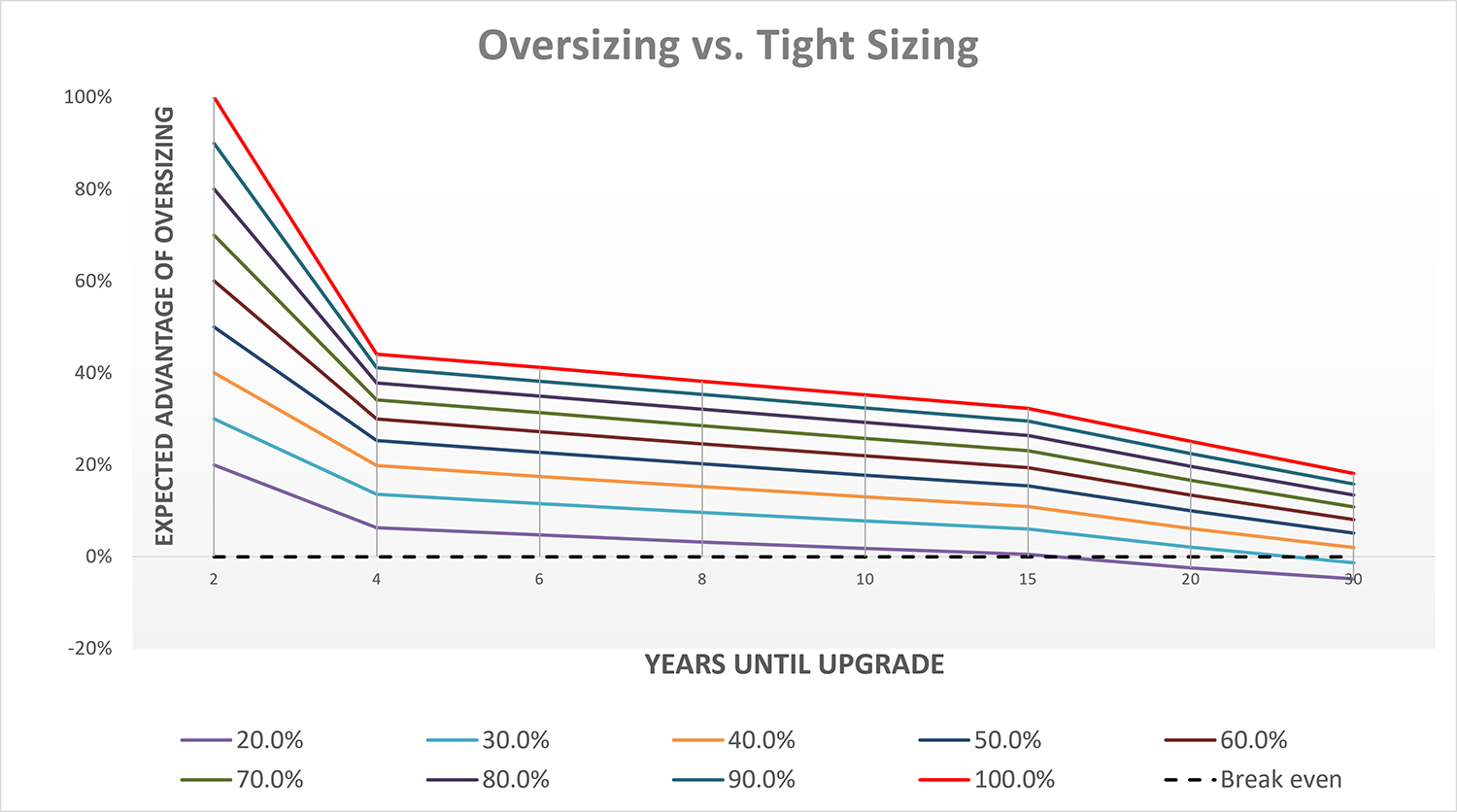
Figure 1 – Break-even pattern. The graph uses the same underlying assumptions as in Table 1: a suburban project area, a weighted-average extra cost of stepping up one dimension of 13%, a service life of 60 years, and a discount rate of 3.5%.
For further information, please contact: Alexander Schou, axsc@cowi.com and Rune Tonell, rune@cowi.com
Network Sizing: A Planning Philosophy, Not Just A Technical Calculation” was published in Hot Cool, edition no. 5/2026. You can download the article here:
Did you find this article useful?
Subscribe to the HOT|COOL newsletters for free and get insightful articles on a variety of topics delivered to your inbox twice a month!